16S rRNA pipeline using DADA2
Instructors: Imane Allali
The dataset
The dataset we will be working are the practice dataset from the H3ABioNet 16S rDNA diversity analysis SOP. The source data can be accessed here but for our purposes it is already on the cluster.
The table below contains the metadata associated with the dog stool samples. There are three dogs which are treated with increased percentage of a compound in their diet: 5 different treatments (0-4, representing an increased percentage of a compound in their diet).
| Sample | Dog | Treatment | Read Counts r1 | Read Counts r2 |
|---|---|---|---|---|
| Dog1 | B | 2 | 118343 | 118343 |
| Dog2 | G | 3 | 108679 | 108679 |
| Dog3 | K | 3 | 101482 | 101482 |
| Dog8 | B | 4 | 108731 | 108731 |
| Dog9 | G | 0 | 109500 | 109500 |
| Dog10 | K | 4 | 79342 | 79342 |
| Dog15 | B | 1 | 131483 | 131483 |
| Dog16 | G | 4 | 114424 | 114424 |
| Dog17 | K | 0 | 99610 | 99610 |
| Dog22 | B | 3 | 145029 | 145029 |
| Dog23 | G | 1 | 193158 | 193158 |
| Dog24 | K | 2 | 162487 | 162487 |
| Dog29 | B | 0 | 122776 | 122776 |
| Dog30 | G | 2 | 137315 | 137315 |
| Dog31 | K | 1 | 150613 | 150613 |
Getting Ready
First, we load the dada2 package on your RStudio. if you do not already have it, see the dada2 installation instructions.
library(dada2); packageVersion("dada2")## [1] '1.13.1'We set the path so that it points to the extracted directory of the dataset named “dog_samples” on your computer or cluster:
MY_HOME <- Sys.getenv("HOME")
data <- paste(MY_HOME, "/dada2_tutorial_dog/dog_samples", sep='')  # change the path
list.files(data)
## [1] "Dog1_R1.fastq" "Dog1_R2.fastq" "Dog10_R1.fastq" "Dog10_R2.fastq"
## [5] "Dog15_R1.fastq" "Dog15_R2.fastq" "Dog16_R1.fastq" "Dog16_R2.fastq"
## [9] "Dog17_R1.fastq" "Dog17_R2.fastq" "Dog2_R1.fastq" "Dog2_R2.fastq"
## [13] "Dog22_R1.fastq" "Dog22_R2.fastq" "Dog23_R1.fastq" "Dog23_R2.fastq"
## [17] "Dog24_R1.fastq" "Dog24_R2.fastq" "Dog29_R1.fastq" "Dog29_R2.fastq"
## [21] "Dog3_R1.fastq" "Dog3_R2.fastq" "Dog30_R1.fastq" "Dog30_R2.fastq"
## [25] "Dog31_R1.fastq" "Dog31_R2.fastq" "Dog8_R1.fastq" "Dog8_R2.fastq"
## [29] "Dog9_R1.fastq" "Dog9_R2.fastq"If your listed files match those here, you can start running the DADA2 pipeline.
Now, we read in the names of the fastq files and we sort them by forward and reverse. Then, we perform some string manipulation to extract a list of the sample names.
# Forward and reverse fastq filenames have format: SAMPLENAME_R1.fastq and SAMPLENAME_R2.fastq
dataF <- sort(list.files(data, pattern="_R1.fastq", full.names = TRUE))
dataR <- sort(list.files(data, pattern="_R2.fastq", full.names = TRUE))

# Extract sample names, assuming filenames have format: SAMPLENAME_XXX.fastq
list.sample.names <- sapply(strsplit(basename(dataF), "_"), `[`, 1)
list.sample.names
## [1] "Dog1" "Dog10" "Dog15" "Dog16" "Dog17" "Dog2" "Dog22" "Dog23"
## [9] "Dog24" "Dog29" "Dog3" "Dog30" "Dog31" "Dog8" "Dog9"1. Quality Control on the Raw Data
The first step of the pipeline consists on visualizing the quality profiles of the dataset.
Here, we visualize the quality profiles of the forward reads:
plotQualityProfile(dataF[1:3])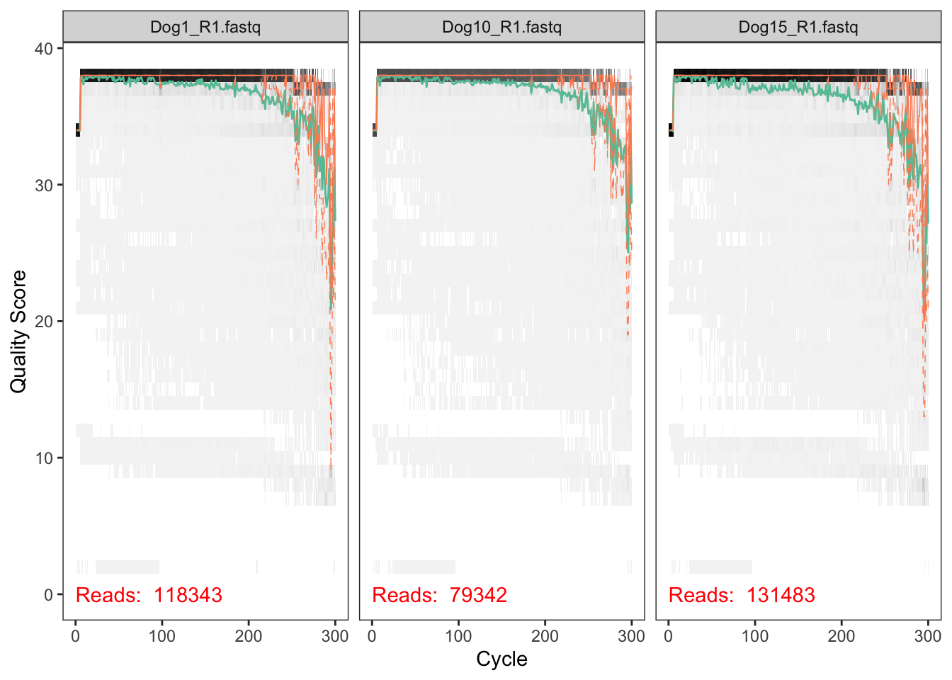
We visualize the quality profiles of the reverse reads:
plotQualityProfile(dataR[1:3])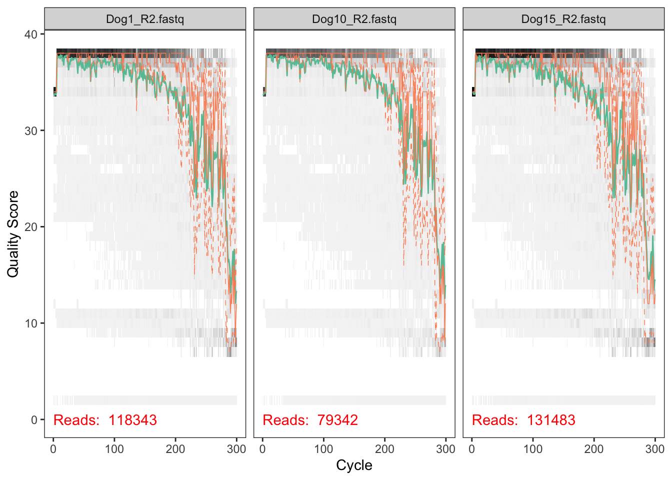
Here, we have only the quality plot for three fastq files you can visualize more plots on the figure.
2. Filter and Trim the Raw Data
We assign the filenames for the filtered "_filt_fastq.gz" files under the filtered/ subdirectory:
# Place filtered files in filtered/ subdirectory
filt.dataF <- file.path(data, "filtered", paste0(list.sample.names, "_F_filt.fastq.gz"))
filt.dataR <- file.path(data, "filtered", paste0(list.sample.names, "_R_filt.fastq.gz"))
names(filt.dataF) <- list.sample.names
names(filt.dataR) <- list.sample.names
For the filtering, we will use these parameters:
maxN = 0 (DADA2 requeris no Ns), truncQ=2, rm.phix=TRUE, maxEE=2 (it is the maximum number of expected errors allowed in a read), truncLen(290, 275) (it depends on the quality of your forward and reverse reads).
out <- filterAndTrim(dataF, filt.dataF, dataR, filt.dataR, truncLen=c(290,275),
              maxN=0, maxEE=c(2,2), truncQ=2, rm.phix=TRUE,
              compress=TRUE, multithread=TRUE) # On Windows set multithread=FALSE
## Creating output directory: /Users/Imane/dada2_tutorial_dog/dog_samples/filteredhead(out)## reads.in reads.out
## Dog1_R1.fastq 118343 84815
## Dog10_R1.fastq 79342 61952
## Dog15_R1.fastq 131483 91235
## Dog16_R1.fastq 114424 83564
## Dog17_R1.fastq 99610 72919
## Dog2_R1.fastq 108679 79668This will take about 3 minutes to run.
3. Learn the Error Rates
The DADA2 pipeline uses the learnErrors method to learn the error model from the data, by alternating the estimation of the error rates and inference of sample composition until they converge on a jointly consistent solution.
We run the error rates on the forward reads:
errF <- learnErrors(filt.dataF, multithread=TRUE)## 114400650 total bases in 394485 reads from 5 samples will be used for learning the error rates.And on the reverse reads:
errR <- learnErrors(filt.dataR, multithread=TRUE)## 108483375 total bases in 394485 reads from 5 samples will be used for learning the error rates.It will take about 30 minutes to run.
Now, we can visualize the estimated error rates for the forward reads:
plotErrors(errF, nominalQ=TRUE)## Warning: Transformation introduced infinite values in continuous y-axis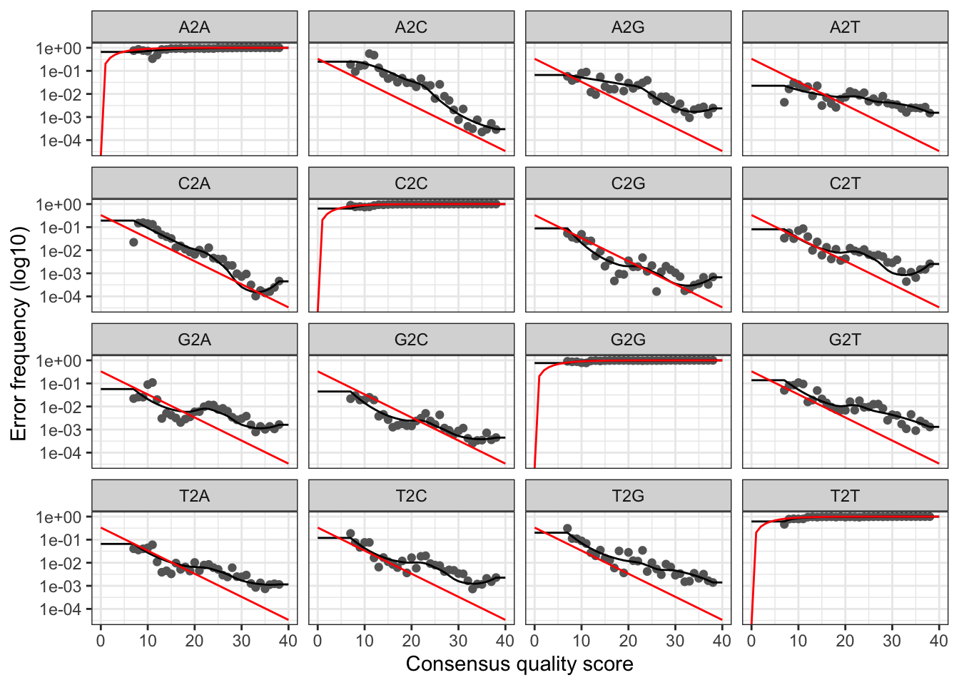
We can visualize the estimated error rates for the reverse reads:
plotErrors(errR, nominalQ=TRUE)## Warning: Transformation introduced infinite values in continuous y-axis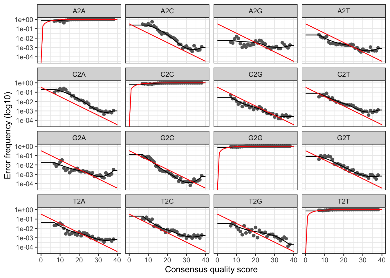
4. Sample Inference
Now, we apply the core sample inference algorithm on the trimmed and filtered forward and reverse reads.
dadaF <- dada(filt.dataF, err=errF, multithread=TRUE)## Sample 1 - 84815 reads in 27400 unique sequences.
## Sample 2 - 61952 reads in 22647 unique sequences.
## Sample 3 - 91235 reads in 25511 unique sequences.
## Sample 4 - 83564 reads in 27549 unique sequences.
## Sample 5 - 72919 reads in 20661 unique sequences.
## Sample 6 - 79668 reads in 27302 unique sequences.
## Sample 7 - 109497 reads in 32980 unique sequences.
## Sample 8 - 151271 reads in 49671 unique sequences.
## Sample 9 - 124140 reads in 38909 unique sequences.
## Sample 10 - 95125 reads in 29652 unique sequences.
## Sample 11 - 76120 reads in 24476 unique sequences.
## Sample 12 - 111204 reads in 38931 unique sequences.
## Sample 13 - 111126 reads in 29513 unique sequences.
## Sample 14 - 78442 reads in 25497 unique sequences.
## Sample 15 - 82843 reads in 28341 unique sequences.dadaR <- dada(filt.dataR, err=errR, multithread=TRUE)## Sample 1 - 84815 reads in 33646 unique sequences.
## Sample 2 - 61952 reads in 24889 unique sequences.
## Sample 3 - 91235 reads in 31503 unique sequences.
## Sample 4 - 83564 reads in 32798 unique sequences.
## Sample 5 - 72919 reads in 25394 unique sequences.
## Sample 6 - 79668 reads in 33192 unique sequences.
## Sample 7 - 109497 reads in 38506 unique sequences.
## Sample 8 - 151271 reads in 55378 unique sequences.
## Sample 9 - 124140 reads in 42968 unique sequences.
## Sample 10 - 95125 reads in 32216 unique sequences.
## Sample 11 - 76120 reads in 27791 unique sequences.
## Sample 12 - 111204 reads in 42880 unique sequences.
## Sample 13 - 111126 reads in 36037 unique sequences.
## Sample 14 - 78442 reads in 30761 unique sequences.
## Sample 15 - 82843 reads in 32614 unique sequences.It will take about 15 minutes to run.
These steps make a dada-class object that can be visualized using the command below:
dadaF[[1]]## dada-class: object describing DADA2 denoising results
## 642 sequence variants were inferred from 27400 input unique sequences.
## Key parameters: OMEGA_A = 1e-40, OMEGA_C = 1e-40, BAND_SIZE = 165. Merge the Paired Reads
In this step, we merge the forward and reverse reads to obtain the full sequences.
merge.reads <- mergePairs(dadaF, filt.dataF, dadaR, filt.dataR, verbose=TRUE)## 76306 paired-reads (in 1153 unique pairings) successfully merged out of 82378 (in 2526 pairings) input.## 54948 paired-reads (in 720 unique pairings) successfully merged out of 60139 (in 1811 pairings) input.## 83013 paired-reads (in 843 unique pairings) successfully merged out of 89310 (in 2175 pairings) input.## 74533 paired-reads (in 1093 unique pairings) successfully merged out of 81135 (in 2674 pairings) input.## 67364 paired-reads (in 855 unique pairings) successfully merged out of 71053 (in 1743 pairings) input.## 69262 paired-reads (in 1194 unique pairings) successfully merged out of 76778 (in 2891 pairings) input.## 97401 paired-reads (in 954 unique pairings) successfully merged out of 106466 (in 2867 pairings) input.## 129237 paired-reads (in 1632 unique pairings) successfully merged out of 146610 (in 5263 pairings) input.## 111558 paired-reads (in 1143 unique pairings) successfully merged out of 120597 (in 3110 pairings) input.## 85319 paired-reads (in 839 unique pairings) successfully merged out of 92957 (in 2348 pairings) input.## 68550 paired-reads (in 915 unique pairings) successfully merged out of 74010 (in 2198 pairings) input.## 92870 paired-reads (in 1266 unique pairings) successfully merged out of 107043 (in 4252 pairings) input.## 101935 paired-reads (in 981 unique pairings) successfully merged out of 108579 (in 2495 pairings) input.## 70424 paired-reads (in 1093 unique pairings) successfully merged out of 75814 (in 2402 pairings) input.## 70177 paired-reads (in 1098 unique pairings) successfully merged out of 79761 (in 3258 pairings) input.Then, we inspect the merger data.frame from the first sample.
head(merge.reads[[1]])## sequence
## 1 TGTGTGCCAGCAGCCGCGGTAATACGGAGGGTGCAAGCGTTAATCGGAATTACTGGGCGTAAAGCGCACGCAGGCGGTTTGTTAAGTCAGATGTGAAATCCCCGGGCTCAACCTGGGAACTGCATCTGATACTGGCAAGCTTGAGTCTCGTAGAGGGGGGTAGAATTCCAGGTGTAGCGGTGAAATGCGTAGAGATCTGGAGGAATACCGGTGGCGAAGGCGGCCCCCTGGACGAAGACTGACGCTCAGGTGCGAAAGCGTGGGGAGCAAACAGGATTAGAAACCCGAGTAGTCCGGCTGACTGACTCGAGA
## 2 TGTGTGCCAGCAGCCGCGGTAATACGGAGGGTGCAAGCGTTAATCGGAATTACTGGGCGTAAAGCGCACGCAGGCGGTTTGTTAAGTCAGATGTGAAATCCCCGGGCTCAACCTGGGAACTGCATCTGATACTGGCAAGCTTGAGTCTCGTAGAGGGGGGTAGAATTCCAGGTGTAGCGGTGAAATGCGTAGAGATCTGGAGGAATACCGGTGGCGAAGGCGGCCCCCTGGACGAAGACTGACGCTCAGGTGCGAAAGCGTGGGGAGCAAACAGGATTAGAAACCCTAGTAGTCCGGCTGACTGACTCGAGA
## 3 TGTGTGCCAGCAGCCGCGGTAATACGGAGGGTGCAAGCGTTAATCGGAATTACTGGGCGTAAAGCGCACGCAGGCGGTTTGTTAAGTCAGATGTGAAATCCCCGGGCTCAACCTGGGAACTGCATCTGATACTGGCAAGCTTGAGTCTCGTAGAGGGGGGTAGAATTCCAGGTGTAGCGGTGAAATGCGTAGAGATCTGGAGGAATACCGGTGGCGAAGGCGGCCCCCTGGACGAAGACTGACGCTCAGGTGCGAAAGCGTGGGGAGCAAACAGGATTAGAAACCCCAGTAGTCCGGCTGACTGACTCGAGA
## 4 TTGTGTGCCAGCAGCCGCGGTAATACGTAGGGGGCTAGCGTTATCCGGATTTACTGGGCGTAAAGGGTGCGTAGGCGGTCTTTCAAGTCAGGAGTTAAAGGCTACGGCTCAACCGTAGTAAGCTCCTGATACTGTCTGACTTGAGTGCAGGAGAGGAAAGCGGAATTCCCAGTGTAGCGGTGAAATGCGTAGATATTGGGAGGAACACCAGTAGCGAAGGCGGCTTTCTGGACTGTAACTGACGCTGAGGCACGAAAGCGTGGGGAGCAAACAGGATTAGAAACCCTAGTAGTCCGGCTGACTGACTCGAGAG
## 5 TGTGTGCCAGCAGCCGCGGTAATACGGAGGGTGCAAGCGTTAATCGGAATTACTGGGCGTAAAGCGCACGCAGGCGGTTTGTTAAGTCAGATGTGAAATCCCCGGGCTCAACCTGGGAACTGCATCTGATACTGGCAAGCTTGAGTCTCGTAGAGGGGGGTAGAATTCCAGGTGTAGCGGTGAAATGCGTAGAGATCTGGAGGAATACCGGTGGCGAAGGCGGCCCCCTGGACGAAGACTGACGCTCAGGTGCGAAAGCGTGGGGAGCAAACAGGATTAGAAACCCTTGTAGTCCGGCTGACTGACTCGAGA
## 6 TGTGTGCCAGCAGCCGCGGTAATACGGAGGGTGCAAGCGTTAATCGGAATTACTGGGCGTAAAGCGCACGCAGGCGGTTTGTTAAGTCAGATGTGAAATCCCCGGGCTCAACCTGGGAACTGCATCTGATACTGGCAAGCTTGAGTCTCGTAGAGGGGGGTAGAATTCCAGGTGTAGCGGTGAAATGCGTAGAGATCTGGAGGAATACCGGTGGCGAAGGCGGCCCCCTGGACGAAGACTGACGCTCAGGTGCGAAAGCGTGGGGAGCAAACAGGATTAGAAACCCTGGTAGTCCGGCTGACTGACTCGAGA
## abundance forward reverse nmatch nmismatch nindel prefer accept
## 1 460 2 1 253 0 0 2 TRUE
## 2 456 1 1 253 0 0 2 TRUE
## 3 421 5 1 253 0 0 2 TRUE
## 4 414 7 2 252 0 0 2 TRUE
## 5 401 6 1 253 0 0 2 TRUE
## 6 400 4 1 253 0 0 2 TRUE6. Construct Sequence Table
We construct the amplicon sequence variant table (ASV):
seqtab <- makeSequenceTable(merge.reads)
dim(seqtab)
## [1] 15 13527We inspect the distribution of sequence lengths:
table(nchar(getSequences(seqtab)))##
## 311 312 313 315
## 107 9136 4283 17. Remove Chimeras
We remove the chimeric ASVs.
seqtab.nochim <- removeBimeraDenovo(seqtab, method="consensus", multithread=TRUE, verbose=TRUE)## Identified 9112 bimeras out of 13527 input sequences.dim(seqtab.nochim)## [1] 15 4415sum(seqtab.nochim)/sum(seqtab)## [1] 0.50949688. Track Reads through the DADA2 Pipeline
In this step, we are going to track the number of reads that made it through each step in the DADA2 pipeline:
getN <- function(x) sum(getUniques(x))
track.nbr.reads <- cbind(out, sapply(dadaF, getN), sapply(dadaR, getN), sapply(merge.reads, getN), rowSums(seqtab.nochim))

colnames(track.nbr.reads) <- c("input", "filtered", "denoisedF", "denoisedR", "merged", "nonchim")
rownames(track.nbr.reads) <- list.sample.names
head(track.nbr.reads)
## input filtered denoisedF denoisedR merged nonchim
## Dog1 118343 84815 82888 83710 76306 35440
## Dog10 79342 61952 60537 61130 54948 24103
## Dog15 131483 91235 89781 90372 83013 48592
## Dog16 114424 83564 81753 82442 74533 46006
## Dog17 99610 72919 71427 72229 67364 42960
## Dog2 108679 79668 77366 78301 69262 301299. Assign Taxonomy
Now, we assign taxonomy to the sequence variants. Before running the command below, download the RefSeq-RDP16S_v3_May2018.fa.gz file from here, and place it in your working directory with the dog samples folder.
taxa <- assignTaxonomy(seqtab.nochim, paste(MY_HOME, "/dada2_tutorial_dog/RefSeq-RDP16S_v3_May2018.fa.gz", sep=''), multithread=TRUE) # change the pathAfter assigning taxonomy, let’s see the results.
taxa.print <- taxa # Removing sequence rownames for display only
rownames(taxa.print) <- NULL
head(taxa.print)
## Kingdom Phylum Class Order
## [1,] "Bacteria" "Firmicutes" "Clostridia" "Clostridiales"
## [2,] "Bacteria" "Firmicutes" "Clostridia" "Clostridiales"
## [3,] "Bacteria" "Bacteroidetes" "Bacteroidia" "Bacteroidales"
## [4,] "Bacteria" "Bacteroidetes" "Bacteroidia" "Bacteroidales"
## [5,] "Bacteria" "Firmicutes" "Clostridia" "Clostridiales"
## [6,] "Bacteria" "Firmicutes" "Clostridia" "Clostridiales"
## Family Genus
## [1,] "Peptostreptococcaceae" "Clostridium_XI"
## [2,] "Peptostreptococcaceae" "Clostridium_XI"
## [3,] "Prevotellaceae" "Alloprevotella"
## [4,] "Prevotellaceae" "Alloprevotella"
## [5,] "Peptostreptococcaceae" "Clostridium_XI"
## [6,] "Peptostreptococcaceae" "Clostridium_XI"
## Species
## [1,] "Clostridium_hiranonis(AB023970)"
## [2,] "Clostridium_hiranonis(AB023970)"
## [3,] "Prevotellamassilia_timonensis(NR_144750.1)"
## [4,] "Prevotellamassilia_timonensis(NR_144750.1)"
## [5,] "Clostridium_hiranonis(AB023970)"
## [6,] "Clostridium_hiranonis(AB023970)"Finally, we can save the ASVs table in your working directory.
write.csv(taxa, file="ASVs_taxonomy.csv")
saveRDS(taxa, "ASVs_taxonomy.rds")
and the ASVs count table.
asv_headers <- vector(dim(seqtab.nochim)[2], mode="character")
count.asv.tab <- t(seqtab.nochim)
row.names(count.asv.tab) <- sub(">", "", asv_headers)
write.csv(count.asv.tab, file="ASVs_counts.csv")
saveRDS(count.asv.tab, file="ASVs_counts.rds")
10. Alignment
Phylogenetic relatedness is commonly used to inform downstream analyses, especially the calculation of phylogeny- aware distances between microbial communities. The DADA2 sequence inference method is reference-free, so we must construct the phylogenetic tree relating the inferred sequence variants de novo. Before constructing the phylogenetic tree. We should do an anlignment. We can perform a multi-alignment using DECIPHER package.
First, we load the package.
library(DECIPHER)Then, we do the alignment. We use the seqtab (sequence table as an input) that we got from step number 6.
seqs <- getSequences(seqtab.nochim)
names(seqs) <- seqs # This propagates to the tip labels of the tree
alignment <- AlignSeqs(DNAStringSet(seqs), anchor=NA)
11. Construct Phylogenetic Tree
After the alignment, we can construct the phylogenetic tree. We use the phangorn package.
First, we load phangorn package.
library(phangorn)If the package is not installed. You can run this command: install.packages(“phangorn”) in your R environment and then load the package.
Here, we first construct a neighbor-joining tree, and then fit a GTR+G+I (Generalized time-reversible with Gamma rate variation) maximum likelihood tree using the neighbor-joining tree as a starting point.
phang.align <- phyDat(as(alignment, "matrix"), type="DNA")
dm <- dist.ml(phang.align)
treeNJ <- NJ(dm) # Note, tip order != sequence order
fit = pml(treeNJ, data=phang.align)
## negative edges length changed to 0!Here, we change the negative edges length to 0. Then, we save the fitGTR file.
fitGTR <- update(fit, k=4, inv=0.2)
fitGTR <- optim.pml(fitGTR, model="GTR", optInv=TRUE, optGamma=TRUE,
rearrangement = "stochastic", control = pml.control(trace = 0))
## Warning in optimize(f = fn, interval = c(0.1, 500), lower = 0.1, upper =
## 500, : NA/Inf replaced by maximum positive value
## Warning in optimize(f = fn, interval = c(0.1, 500), lower = 0.1, upper =
## 500, : NA/Inf replaced by maximum positive value
## Warning in optimize(f = fn, interval = c(0.1, 500), lower = 0.1, upper =
## 500, : NA/Inf replaced by maximum positive value
## Warning in optimize(f = fn, interval = c(0.1, 500), lower = 0.1, upper =
## 500, : NA/Inf replaced by maximum positive value
## Warning in optimize(f = fn, interval = c(0.1, 500), lower = 0.1, upper =
## 500, : NA/Inf replaced by maximum positive value
## Warning in optimize(f = fn, interval = c(0.1, 500), lower = 0.1, upper =
## 500, : NA/Inf replaced by maximum positive value
## Warning in optimize(f = fn, interval = c(0.1, 500), lower = 0.1, upper =
## 500, : NA/Inf replaced by maximum positive value
## Warning in optimize(f = fn, interval = c(0.1, 500), lower = 0.1, upper =
## 500, : NA/Inf replaced by maximum positive value
## Warning in optimize(f = fn, interval = c(0.1, 500), lower = 0.1, upper =
## 500, : NA/Inf replaced by maximum positive value
## Warning in optimize(f = fn, interval = c(0.1, 500), lower = 0.1, upper =
## 500, : NA/Inf replaced by maximum positive value
## Warning in optimize(f = fn, interval = c(0.1, 500), lower = 0.1, upper =
## 500, : NA/Inf replaced by maximum positive value
## Warning in optimize(f = fn, interval = c(0.1, 500), lower = 0.1, upper =
## 500, : NA/Inf replaced by maximum positive value
## Warning in optimize(f = fn, interval = c(0.1, 500), lower = 0.1, upper =
## 500, : NA/Inf replaced by maximum positive value
## Warning in optimize(f = fn, interval = c(0.1, 500), lower = 0.1, upper =
## 500, : NA/Inf replaced by maximum positive value
## Warning in optimize(f = fn, interval = c(0.1, 500), lower = 0.1, upper =
## 500, : NA/Inf replaced by maximum positive value
## Warning in optimize(f = fn, interval = c(0.1, 500), lower = 0.1, upper =
## 500, : NA/Inf replaced by maximum positive value
## Warning in optimize(f = fn, interval = c(0.1, 500), lower = 0.1, upper =
## 500, : NA/Inf replaced by maximum positive value
## Warning in optimize(f = fn, interval = c(0.1, 500), lower = 0.1, upper =
## 500, : NA/Inf replaced by maximum positive value
## Warning in optimize(f = fn, interval = c(0.1, 500), lower = 0.1, upper =
## 500, : NA/Inf replaced by maximum positive value
## Warning in optimize(f = fn, interval = c(0.1, 500), lower = 0.1, upper =
## 500, : NA/Inf replaced by maximum positive value
## Warning in optimize(f = fn, interval = c(0.1, 500), lower = 0.1, upper =
## 500, : NA/Inf replaced by maximum positive value
## Warning in optimize(f = fn, interval = c(0.1, 500), lower = 0.1, upper =
## 500, : NA/Inf replaced by maximum positive value
## Warning in optimize(f = fn, interval = c(0.1, 500), lower = 0.1, upper =
## 500, : NA/Inf replaced by maximum positive value
## Warning in optimize(f = fn, interval = c(0.1, 500), lower = 0.1, upper =
## 500, : NA/Inf replaced by maximum positive value
## Warning in optimize(f = fn, interval = c(0.1, 500), lower = 0.1, upper =
## 500, : NA/Inf replaced by maximum positive value
## Warning in optimize(f = fn, interval = c(0.1, 500), lower = 0.1, upper =
## 500, : NA/Inf replaced by maximum positive value
## Warning in optimize(f = fn, interval = c(0.1, 500), lower = 0.1, upper =
## 500, : NA/Inf replaced by maximum positive value
## Warning in optimize(f = fn, interval = c(0.1, 500), lower = 0.1, upper =
## 500, : NA/Inf replaced by maximum positive value
## Warning in optimize(f = fn, interval = c(0.1, 500), lower = 0.1, upper =
## 500, : NA/Inf replaced by maximum positive value
## Warning in optimize(f = fn, interval = c(0.1, 500), lower = 0.1, upper =
## 500, : NA/Inf replaced by maximum positive value
## Warning in optimize(f = fn, interval = c(0.1, 500), lower = 0.1, upper =
## 500, : NA/Inf replaced by maximum positive value
## Warning in optimize(f = fn, interval = c(0.1, 500), lower = 0.1, upper =
## 500, : NA/Inf replaced by maximum positive value
## Warning in optimize(f = fn, interval = c(0.1, 500), lower = 0.1, upper =
## 500, : NA/Inf replaced by maximum positive value
## Warning in optimize(f = fn, interval = c(0.1, 500), lower = 0.1, upper =
## 500, : NA/Inf replaced by maximum positive value
## Warning in optimize(f = fn, interval = c(0.1, 500), lower = 0.1, upper =
## 500, : NA/Inf replaced by maximum positive value
## Warning in optimize(f = fn, interval = c(0.1, 500), lower = 0.1, upper =
## 500, : NA/Inf replaced by maximum positive value
## Warning in optimize(f = fn, interval = c(0.1, 500), lower = 0.1, upper =
## 500, : NA/Inf replaced by maximum positive value
## Warning in optimize(f = fn, interval = c(0.1, 500), lower = 0.1, upper =
## 500, : NA/Inf replaced by maximum positive value
## Warning in optimize(f = fn, interval = c(0.1, 500), lower = 0.1, upper =
## 500, : NA/Inf replaced by maximum positive value
## Warning in optimize(f = fn, interval = c(0.1, 500), lower = 0.1, upper =
## 500, : NA/Inf replaced by maximum positive value
## Warning in optimize(f = fn, interval = c(0.1, 500), lower = 0.1, upper =
## 500, : NA/Inf replaced by maximum positive value
## Warning in optimize(f = fn, interval = c(0.1, 500), lower = 0.1, upper =
## 500, : NA/Inf replaced by maximum positive value
## Warning in optimize(f = fn, interval = c(0.1, 500), lower = 0.1, upper =
## 500, : NA/Inf replaced by maximum positive value
## Warning in optimize(f = fn, interval = c(0.1, 500), lower = 0.1, upper =
## 500, : NA/Inf replaced by maximum positive value
## Warning in optimize(f = fn, interval = c(0.1, 500), lower = 0.1, upper =
## 500, : NA/Inf replaced by maximum positive value
## Warning in optimize(f = fn, interval = c(0.1, 500), lower = 0.1, upper =
## 500, : NA/Inf replaced by maximum positive value
## Warning in optimize(f = fn, interval = c(0.1, 500), lower = 0.1, upper =
## 500, : NA/Inf replaced by maximum positive value
## Warning in optimize(f = fn, interval = c(0.1, 500), lower = 0.1, upper =
## 500, : NA/Inf replaced by maximum positive value
## Warning in optimize(f = fn, interval = c(0.1, 500), lower = 0.1, upper =
## 500, : NA/Inf replaced by maximum positive value
## Warning in optimize(f = fn, interval = c(0.1, 500), lower = 0.1, upper =
## 500, : NA/Inf replaced by maximum positive value
## Warning in optimize(f = fn, interval = c(0.1, 500), lower = 0.1, upper =
## 500, : NA/Inf replaced by maximum positive value
## Warning in optimize(f = fn, interval = c(0.1, 500), lower = 0.1, upper =
## 500, : NA/Inf replaced by maximum positive value
## Warning in optimize(f = fn, interval = c(0.1, 500), lower = 0.1, upper =
## 500, : NA/Inf replaced by maximum positive value
## Warning in optimize(f = fn, interval = c(0.1, 500), lower = 0.1, upper =
## 500, : NA/Inf replaced by maximum positive value
## Warning in optimize(f = fn, interval = c(0.1, 500), lower = 0.1, upper =
## 500, : NA/Inf replaced by maximum positive value
## Warning in optimize(f = fn, interval = c(0.1, 500), lower = 0.1, upper =
## 500, : NA/Inf replaced by maximum positive value
## Warning in optimize(f = fn, interval = c(0.1, 500), lower = 0.1, upper =
## 500, : NA/Inf replaced by maximum positive value
## Warning in optimize(f = fn, interval = c(0.1, 500), lower = 0.1, upper =
## 500, : NA/Inf replaced by maximum positive value
## Warning in optimize(f = fn, interval = c(0.1, 500), lower = 0.1, upper =
## 500, : NA/Inf replaced by maximum positive value
## Warning in optimize(f = fn, interval = c(0.1, 500), lower = 0.1, upper =
## 500, : NA/Inf replaced by maximum positive value
## Warning in optimize(f = fn, interval = c(0.1, 500), lower = 0.1, upper =
## 500, : NA/Inf replaced by maximum positive value
## Warning in optimize(f = fn, interval = c(0.1, 500), lower = 0.1, upper =
## 500, : NA/Inf replaced by maximum positive value
## Warning in optimize(f = fn, interval = c(0.1, 500), lower = 0.1, upper =
## 500, : NA/Inf replaced by maximum positive value
## Warning in optimize(f = fn, interval = c(0.1, 500), lower = 0.1, upper =
## 500, : NA/Inf replaced by maximum positive value
## Warning in optimize(f = fn, interval = c(0.1, 500), lower = 0.1, upper =
## 500, : NA/Inf replaced by maximum positive value
## Warning in optimize(f = fn, interval = c(0.1, 500), lower = 0.1, upper =
## 500, : NA/Inf replaced by maximum positive value
## Warning in optimize(f = fn, interval = c(0.1, 500), lower = 0.1, upper =
## 500, : NA/Inf replaced by maximum positive value
## Warning in optimize(f = fn, interval = c(0.1, 500), lower = 0.1, upper =
## 500, : NA/Inf replaced by maximum positive value
## Warning in optimize(f = fn, interval = c(0.1, 500), lower = 0.1, upper =
## 500, : NA/Inf replaced by maximum positive value
## Warning in optimize(f = fn, interval = c(0.1, 500), lower = 0.1, upper =
## 500, : NA/Inf replaced by maximum positive value
## Warning in optimize(f = fn, interval = c(0.1, 500), lower = 0.1, upper =
## 500, : NA/Inf replaced by maximum positive value
## Warning in optimize(f = fn, interval = c(0.1, 500), lower = 0.1, upper =
## 500, : NA/Inf replaced by maximum positive value
## Warning in optimize(f = fn, interval = c(0.1, 500), lower = 0.1, upper =
## 500, : NA/Inf replaced by maximum positive valuesaveRDS(fitGTR, "phangorn.tree.RDS")